Differential Evolution

Evolutionary Algorithms - Differential Evolution

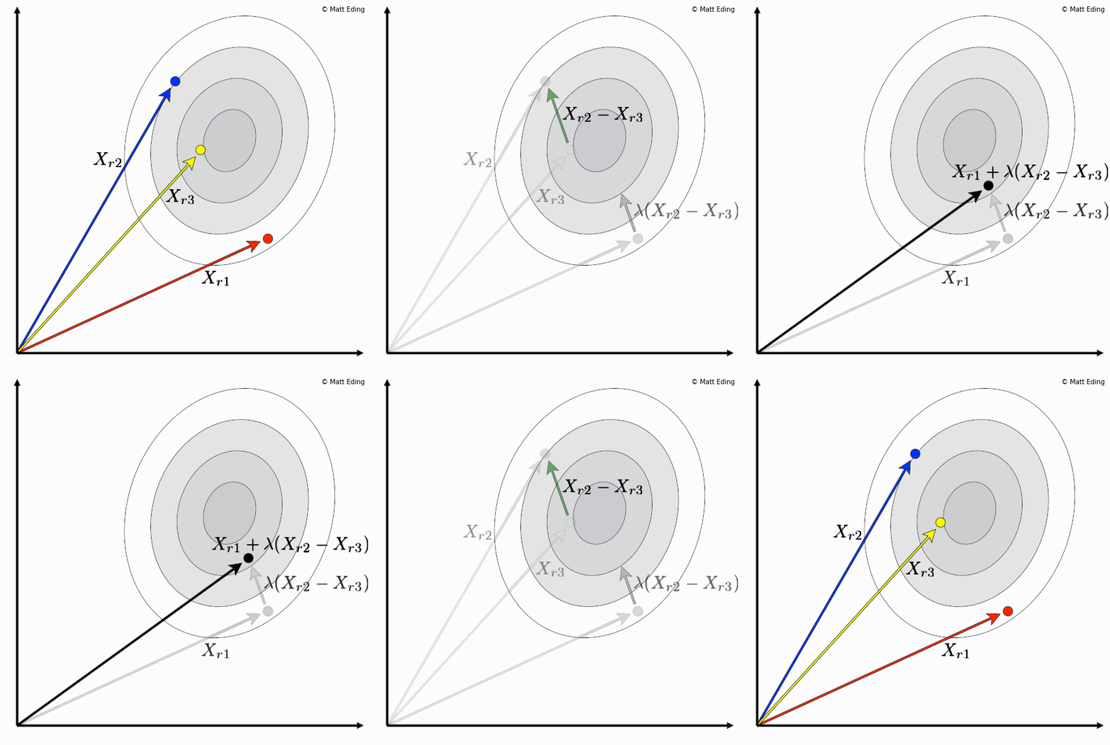
Differential evolution is a method to create new chromosomes for a population. While iterating over generations to evolve to an optimal state, we use existing chromosomes to create offspring as potential candidates to make it to the next generation. The steps of differential evolution is as follows:

1. For each chromosome in the population you select three other distinct members.
2. If a uniformly random number from 0 to 1 is less than the user defined crossover rate, create a new offspring vector. Otherwise use the same chromosome as the parent.
3. Subtract two of these chromosome vectors.
4. Scale the difference by a user defined hyperparameter λ.
5. Add the scaled vector to the third chromosome.

If the resulting offspring has a better fitness score than its parent chromosome, it will replace its parent for the subsequent generation. Below is an implementation to create the offspring using NumPy:

Create an initial population randomly. For sake of example, the normal distribution is used. Typically there would be other constraints for the population. Note that each row is interpreted as a chromosome.

In [1]: import numpy as np

In [2]: pop = np.random.normal(size=(10, 4))

In [3]: pop
Out[3]:
array([[-0.64253779, -2.39215419,  0.79103703,  1.23892021],
       [ 0.65684701, -0.88219666, -0.23691506,  1.61460243],
       [ 1.4740972 , -1.09393222, -0.73541817,  0.27248896],
       [ 0.62403672, -1.22836506,  1.08530489,  0.81942899],
       [-0.46313748, -0.61334157, -1.29684186,  1.06648673],
       [ 0.79976224,  1.1295049 ,  0.3129676 , -0.74281539],
       [-0.43466301, -1.25084627,  0.54151209, -0.51814957],
       [ 0.45798788,  0.8910426 ,  1.71402891,  0.62185348],
       [-0.35507422, -0.74275952, -0.5113616 ,  1.69085342],
       [-0.43192986, -0.07482148,  0.33823173,  0.97419619]])

Choose values for hyperparameters. The crossover rate is a percentage as a decimal. The value for λ is usually in the interval of [0, 1] but can take on other values.

In [4]: crossover = 0.5

In [5]: lam = 0.7

Here are two different implementations for choosing the three distinct chromosomes. While I find the first method is easier to read, the second version is over twice as fast. Regardless of whichever you choose, the results are the same. np.squeeze is used to remove the excess dimension created from splitting the array of chromosomes selected from the population into three columns.

In [6]: %%timeit  # version 1
   ...: arr = np.arange(len(pop))
   ...: idxs = np.array([np.random.choice(np.setdiff1d(arr, i), size=3, replace=False)
   ...:                  for i in arr])
# 459 µs ± 21.2 µs per loop (mean ± std. dev. of 7 runs, 1000 loops each)

In [7]: %%timeit  # version 2
   ...: frzn = frozenset(range(len(pop)))
   ...: idxs = np.array([np.random.choice(tuple(frzn - {i}), size=3, replace=False)
   ...:                  for i in frzn])
# 187 µs ± 704 ns per loop (mean ± std. dev. of 7 runs, 10000 loops each)

In [8]: chrom_1, chrom_2, chrom_3 = map(np.squeeze, np.split(pop[idxs], 3, axis=1))

Confirm all selected chromosomes are indeed distinct from each other.

In [9]: from itertools import combinations

In [11]: combos = combinations([pop, chrom_1, chrom_2, chrom_3], r=2)

In [12]: assert not np.any([np.any(chrom_x == chrom_y, axis=1)
    ...:                    for chrom_x, chrom_y in combos])

Create candidate offspring chromosomes according to steps 3-5 above. Then use a mask to implement step 2, where some chromosomes of the parent population are to be kept.

In [13]: offspr = (chrom_1 + lam * (chrom_2 - chrom_3))

In [14]: rand = np.random.random_sample(len(pop))

In [15]: mask = rand > crossover

In [16]: offspr[mask] = pop[mask]

In [17]: offspr
Out[17]:
array([[-1.74355748, -2.39215419, -1.14000226,  2.05934185],
       [ 2.10568121, -0.31960968,  0.01678626,  0.14292712],
       [ 1.4740972 , -1.09393222, -0.73541817,  0.27248896],
       [ 0.62403672, -1.22836506,  1.08530489,  0.81942899],
       [ 0.19292576,  1.42450074,  1.1589935 ,  1.06648673],
       [ 1.34459004,  1.70569499,  1.92001642, -0.74281539],
       [-0.43466301, -1.25084627,  0.54151209, -0.51814957],
       [ 0.45798788,  0.8910426 ,  1.71402891,  0.62185348],
       [-0.35507422, -0.74275952, -0.5113616 ,  1.69085342],
       [-1.9163075 , -2.15960166,  0.33823173,  0.1583523 ]])

As seen in the resulting offspring, there are chromosomes (rows) that are the same as the original population. The others are completely new chromosomes to offer variation during the evolution process to prevent the algorithm from being stuck in local minima.

A nice property of differential evolution is that unlike using gradient descent as an optimizer, it does not require differentiability. However it should be mentioned that while this optimization method does not guarantee the best solution, it still does a very job at finding solutions. It is only a matter of comparing the fitness scores to determine which of the offspring or parent chromosomes make it to the next generation. But maybe that, mutation, and more will be a future topic for another day.

In [18]: exit()  # the end :D

Code used to create the above animation is located at my GitHub.