Numpy Broadcasting
NumPy - Broadcasting
NumPy has an awesome feature known as broadcasting. This feature allows users to perform operations between an array and another array or a scalar. Conceptually, NumPy expands the arrays until their shapes match (if possible). The rule to determine whether two arrays can be broadcasted is:
Corresponding axes must be equal or 1 when the shapes are right-aligned.
Here is an example of the rule working:
In [1]: import numpy as np

In [2]: arr_1 = np.zeros(shape=(2, 5, 3, 7, 10))

In [3]: arr_2 = np.full(shape=(3, 1, 10), fill_value=np.nan)

In [4]: shapes = [str(a.shape) for a in (arr_1, arr_2)]

In [5]: longest = len(max(shapes, key=len))

In [6]: rjusts = [s.rjust(longest) for s in shapes]

In [7]: print(*rjusts, sep='\n')
# (2, 5, 3, 7, 10)
#       (3, 1, 10)
Looking at the above output:
- The first two columns do not have corresponding values in the second row. The missing values will be created and expanded into 2 and 5.
- The middle and last columns have equal values between the two shapes. These axes will not be expanded.
- The remaining column has values 7 and 1. While the values are not equal, the 1 will be expanded into 7.
Here is an example that fails to broadcast:
In [8]: arr_3 = np.array([[[4, 2, 1]]])

In [9]: arr_4 = (np.linspace(0, 100, 12)  # 12 equally spaced numbers from 0 to 100
   ...:            .reshape(-1, 6)  # -1 has numpy calculate first axis dimension
   ...:            .astype(int))

In [10]: arr_3 - arr_4
# ValueError: operands could not be broadcast together with shapes (2,6) (1,1,3)
With shape (1, 1, 3), the two 1’s are ok since the first has no corresponding value and the second is a 1. It is the final axis with 6 and 3 that cause the error; they are not equal and neither are 1. NumPy will not venture to guess whether it should double the 3 to a 6. If this is what you wanted, you would need to manually extend them:
In [11]: np.dstack((arr_3, arr_3)) - arr_4  # stack extra copy depth-wise
Out[11]:
array([[[  4,  -7, -17, -23, -34, -44],
        [-50, -61, -71, -77, -88, -99]]])

In [12]: _.shape  # ipython previous output
Out[12]: (1, 2, 6)
While the notion of expansion is helpful to understand broadcasting, NumPy does not actually create new, bigger arrays. This allows NumPy to be more efficient in both speed…
In [13]: nums = np.arange(1e6).reshape(10, 10, -1)  # -1 has numpy calculate third axis dimension

In [14]: ones = np.ones_like(nums)  # same shape with np.*_like functions

In [15]: %timeit nums + 1
# 1.01 ms ± 5.15 µs per loop (mean ± std. dev. of 7 runs, 1000 loops each)

In [16]: %timeit nums + ones
# 1.14 ms ± 8.1 µs per loop (mean ± std. dev. of 7 runs, 1000 loops each)
… and memory since an array of only unique values needs to allocate space for all the values (even when taking dtypes into consideration).
In [17]: (1).__sizeof__()
# 24

In [18]: ones.__sizeof__()
# 800128

In [19]: np.array_equal(nums + 1, nums + ones)
Out[19]: True
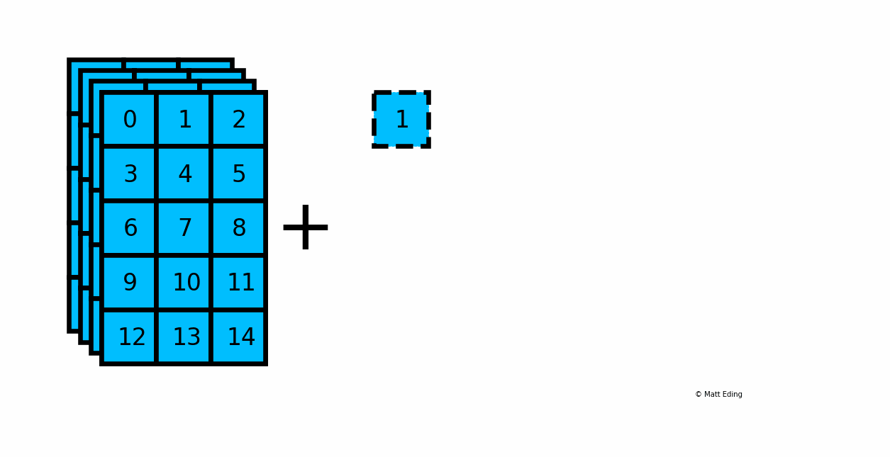
Below is an example of adding a scalar to a 3D array:
In [20]: arr_3d = np.arange(60).reshape(5, 3, 4)

In [21]: np.shape(arr_3d)
Out[21]: (5, 3, 4)

In [22]: np.shape(1)
Out[22]: ()

In [23]: result = arr_3d + 1

In [24]: np.shape(result)
Out[24]: (5, 3, 4)
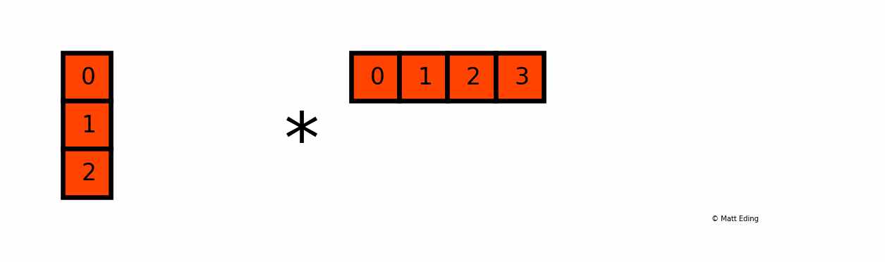
Another example with multiplying a column by a row:
In [25]: np.c_[0:3]  # create column with slice syntax
Out[25]:
array([[0],
       [1],
       [2]])

In [26]: np.r_[0:4]  # create row with slice syntax
Out[26]: array([0, 1, 2, 3])

In [27]: _ * __  # ipython previous two outputs
Out[27]:
array([[0, 0, 0, 0],
       [0, 1, 2, 3],
       [0, 2, 4, 6]])
An application in data science using broadcasting is the ability to normalize data to range from 0 to 1.
In [28]: data = np.array([[ 4.4,  2.1, -9.0],
    ...:                  [ 0.4, -3.2,  3.9],
    ...:                  [-6.7, -5.0,  7.4]])

In [29]: data -= data.min()  # make min value 0

In [30]: data /= data.max()  # make max value 1

In [31]: assert (data.min() == 0) and (data.max() == 1)

In [32]: data
Out[32]:
array([[0.81707317, 0.67682927, 0.        ],
       [0.57317073, 0.35365854, 0.78658537],
       [0.1402439 , 0.24390244, 1.        ]])
Hopefully this will help you embrace using the power of broadcasting in your future work. It allows you to concisely write code (i.e. less error prone) while making your program more performant at the same time.
In [33]: exit() # the end :D
Code used to create the above animations are located at my GitHub.