Sparse Matrices
Data Structures - Sparse Matrices
Table of Contents
- Introduction
- Construction Matrices
- Compressed Sparse Matrices
- Diagonal Matrix
- Specialized Functions
- Other Libraries
- Final Thoughts
Introduction
A sparse matrix is a matrix that has a value of 0 for most elements. If the ratio of Number of Non-Zero (NNZ) elements to the size is less than 0.5, the matrix is sparse. While this is the mathematical definition, I will be using the term sparse for matrices with only NNZ elements and dense for matrices with all elements.
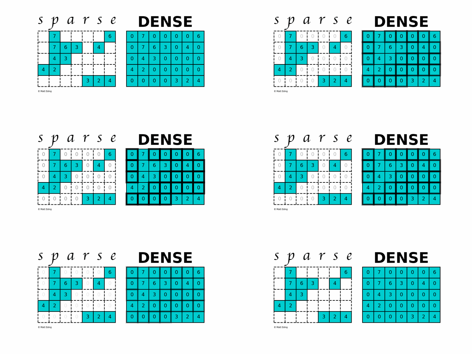
Storing information about all the 0 elements is inefficient, so we will assume unspecified elements to be 0. Using this scheme, sparse matrices can perform faster operations and use less memory than its corresponding dense matrix representation, which is especially important when working with large data sets in data science.
Today we will investigate all of the different implementations provided by the SciPy sparse package.
This implementation is modeled after np.matrix opposed to np.ndarray, thus is restricted to 2-D arrays and having quirks like A * B doing matrix multiplication instead of element-wise multiplication.
In [0]: from scipy import sparse

In [1]: import numpy as np

In [2]: spmatrix = sparse.random(10, 10)

In [3]: spmatrix
Out[3]:
<10x10 sparse matrix of type '<class 'numpy.float64'>'
        with 1 stored elements in COOrdinate format>

In [4]: spmatrix.nnz / np.product(spmatrix.shape)  # sparsity
Out[4]: 0.01
Construction Matrices
Different sparse formats have their strengths and weaknesses. A good starting point is looking at formats that are efficient for constructing these matrices. Typically you would start with one of these forms and then convert to another when ready to do calculations.
Coordinate Matrix
Perhaps the simplest sparse format to understand is the COOrdinate (COO) format. This variant uses three subarrays to store the element values and their coordinate positions.
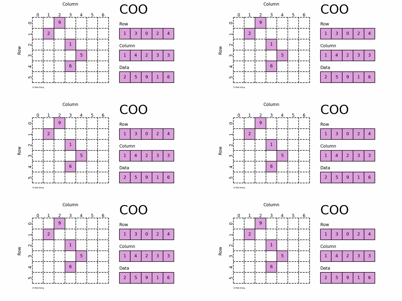
In [5]: row = [1, 3, 0, 2, 4]

In [6]: col = [1, 4, 2, 3, 3]

In [7]: data = [2, 5, 9, 1, 6]

In [8]: coo = sparse.coo_matrix((data, (row, col)), shape=(6, 7))

In [9]: print(coo)  # coordinate-value format
# (1, 1)        2
# (3, 4)        5
# (0, 2)        9
# (2, 3)        1
# (4, 3)        6

In [10]: coo.todense()  # coo.toarray() for ndarray instead
Out[10]:
matrix([[0, 0, 9, 0, 0, 0, 0],
        [0, 2, 0, 0, 0, 0, 0],
        [0, 0, 0, 1, 0, 0, 0],
        [0, 0, 0, 0, 5, 0, 0],
        [0, 0, 0, 6, 0, 0, 0],
        [0, 0, 0, 0, 0, 0, 0]])
The savings on memory consumption is quite substantial as the matrix size increases. Managing data in a sparse structure is a fixed cost unlike the case for dense matrices. The overhead incurred from needing to manage the subarrays is becomes negligible as data grows making it a great choice for some datasets.
A word of caution: only use sparse arrays if they are sufficiently sparse enough; it would be counterproductive storing a mostly nonzero array using several subarrays to keep track of position and data.
In [11]: def memory_usage(coo):
    ...:    # data memory and overhead memory
    ...:    coo_mem = (sum(obj.nbytes for obj in [coo.data, coo.row, coo.col])
    ...:               + sum(obj.__sizeof__() for obj in [coo, coo.data, coo.row, coo.col]))
    ...:    print(f'Sparse: {coo_mem}')
    ...:    mtrx = coo.todense()
    ...:    mtrx_mem = mtx.nbytes + mtrx.__sizeof__()
    ...:    print(f'Dense: {mtrx_mem}')

In [12]: memory_usage(coo)
# Sparse: 480
# Dense: 448

In [13]: coo.resize(100, 100)

In [14]: memory_usage(coo)
# Sparse: 480
# Dense: 80112
Dictionary of Keys Matrix
Dictionary Of Keys (DOK)
is very much like COO except that it subclasses dict to store coordinate-data information as key-value pairs.
Since it uses a hash table as storage, identifying values at any given location has constant lookup time.
Use this format if you need the functionality that come with builtin dictionaries, but be mindful that hash tables hog much more memory than arrays.
In [15]: dok = sparse.dok_matrix((10, 10))

In [16]: dok[(3, 7)] = 42  # store value 42 at coordinate (3, 7)

In [17]: dok[(9, 5)]  # zero elements are accessible
Out[17]: 0.0

In [18]: dok.keys() | dok.transpose().keys()  # union of key views
Out[18]: {(3, 7), (7, 3)}

In [19]: isinstance(dok, dict)
Out[19]: True
Note: be careful of potential problems using the methods inherited from dict; they don’t always behave.
In [20]: out_of_bounds = (999, 999)

In [21]: dok[out_of_bounds] = 1  # works as expected
IndexError: Index out of bounds.

In [22]: dok.setdefault(out_of_bounds)  # silently ignored...

In [23]: dok.toarray()  # ...until now
ValueError: row index exceeds matrix dimensions

In [24]: dok.pop(out_of_bounds)  # fix issue by removing bad point

In [25]: sparse.dok_matrix.fromkeys([..., ..., ...])  # don't get me started
TypeError: __init__() missing 1 required positional argument: 'arg1'
Linked List Matrix
The most flexible format to insert data is through usage of LInked List (LIL) matrices. Data can be set via indexing and slicing syntax of NumPy to quickly populate the matrix. In my opinion, LIL is the coolest sparse format for constructing sparse matrices from scratch.
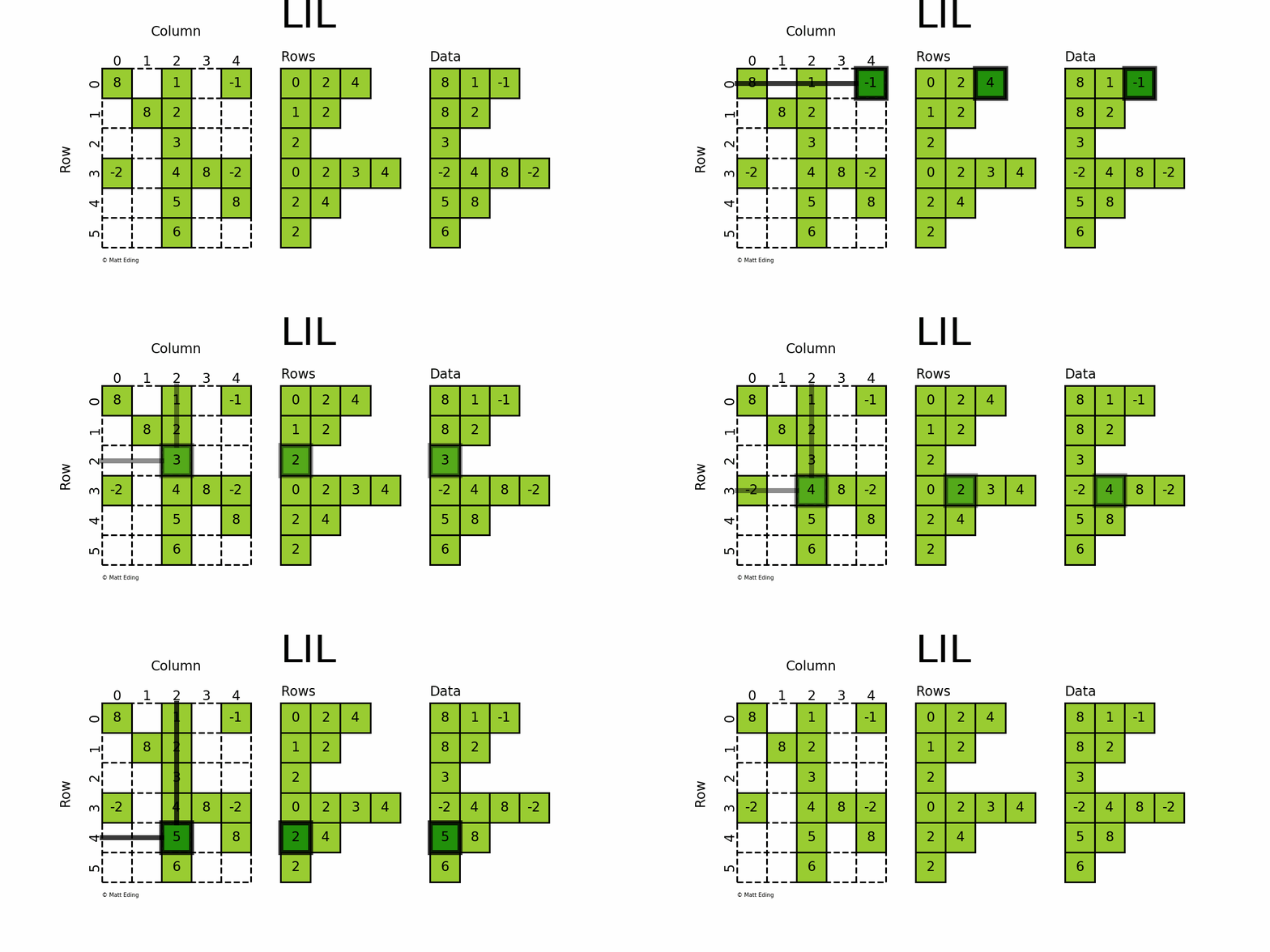
LIL stores information in lil.rows where each list represents a row index and the elements inside the list match columns.
In a parallel array, lil.data, the NNZ values are stored.
But unlike other sparse formats, these subarrays cannot be explicitly passed to the constructor; LIL matrices must be made from either an empty state or from existing matrices, dense or sparse.
Below is an illustration of various techniques used to build up a LIL matrix.
In [26]: lil = sparse.lil_matrix((6, 5), dtype=int)

In [27]: lil[(0, -1)] = -1  # set individual point

In [28]: lil[3, (0, 4)] = [-2] * 2  # set two points

In [29]: lil.setdiag(8, k=0)  # set main diagonal

In [30]: lil[:, 2] = np.arange(lil.shape[0]).reshape(-1, 1) + 1  # set entire column

In [31]: lil.toarray()
Out[31]:
array([[ 8,  0,  1,  0, -1],
       [ 0,  8,  2,  0,  0],
       [ 0,  0,  3,  0,  0],
       [-2,  0,  4,  8, -2],
       [ 0,  0,  5,  0,  8],
       [ 0,  0,  6,  0,  0]])
So what’s the drawback…? Well, it utilizes jagged arrays under the hood which requires np.dtype(object).
This costs a lot more memory than a rectangular array, so if the data is big enough, you may be forced to work with COO instead of LIL.
In short, LIL is mostly offered as a convenience, albeit an awesome one at that.
In [32]: lil.rows
Out[32]:
array([list([0, 2, 4]), list([1, 2]), list([2]), list([0, 2, 3, 4]),
       list([2, 4]), list([2])], dtype=object)

In [33]: lil.data[:, np.newaxis]  # expose jagged structure
Out[33]:
array([[list([8, 1, -1])],
       [list([8, 2])],
       [list([3])],
       [list([-2, 4, 8, -2])],
       [list([5, 8])],
       [list([6])]], dtype=object)
As an aside, Linked List Matrix is a misnomer since it does not use linked lists behind the scenes!
LIL actually uses Python’s list which is a dynamic array, so it should really be called a List of Lists Matrix, in spite of what the documentation says.
(A missed opportunity to christen it as LOL…)
In [34]: sparse.lil.__doc__  # module docstring
Out[34]: 'LInked List sparse matrix class\n'
Compressed Sparse Matrices
The formats described earlier are great for building sparse matrices, but they aren’t as computationally performant than more specialized forms. The reverse is true for compressed sparse matrix family, which should be treated as read-only rather than write-only. These are more difficult to understand, but with a little patience their structure can be grokked.
Compressed Sparse Row/Column
The Compressed Sparse Row/Column (CSR and CSC) formats are designed for computation in mind.
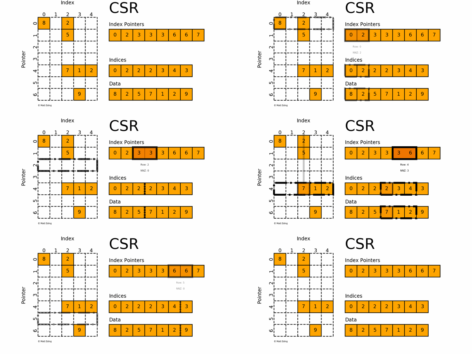
In [35]: indptr = np.array([0, 2, 3, 3, 3, 6, 6, 7])

In [36]: indices = np.array([0, 2, 2, 2, 3, 4, 3])

In [37]: data = np.array([8, 2, 5, 7, 1, 2, 9])

In [38]: csr = sparse.csr_matrix((data, indices, indptr))

In [39]: csr.todense()
Out[39]:
matrix([[8, 0, 2, 0, 0],
        [0, 0, 5, 0, 0],
        [0, 0, 0, 0, 0],
        [0, 0, 0, 0, 0],
        [0, 0, 7, 1, 2],
        [0, 0, 0, 0, 0],
        [0, 0, 0, 9, 0]])
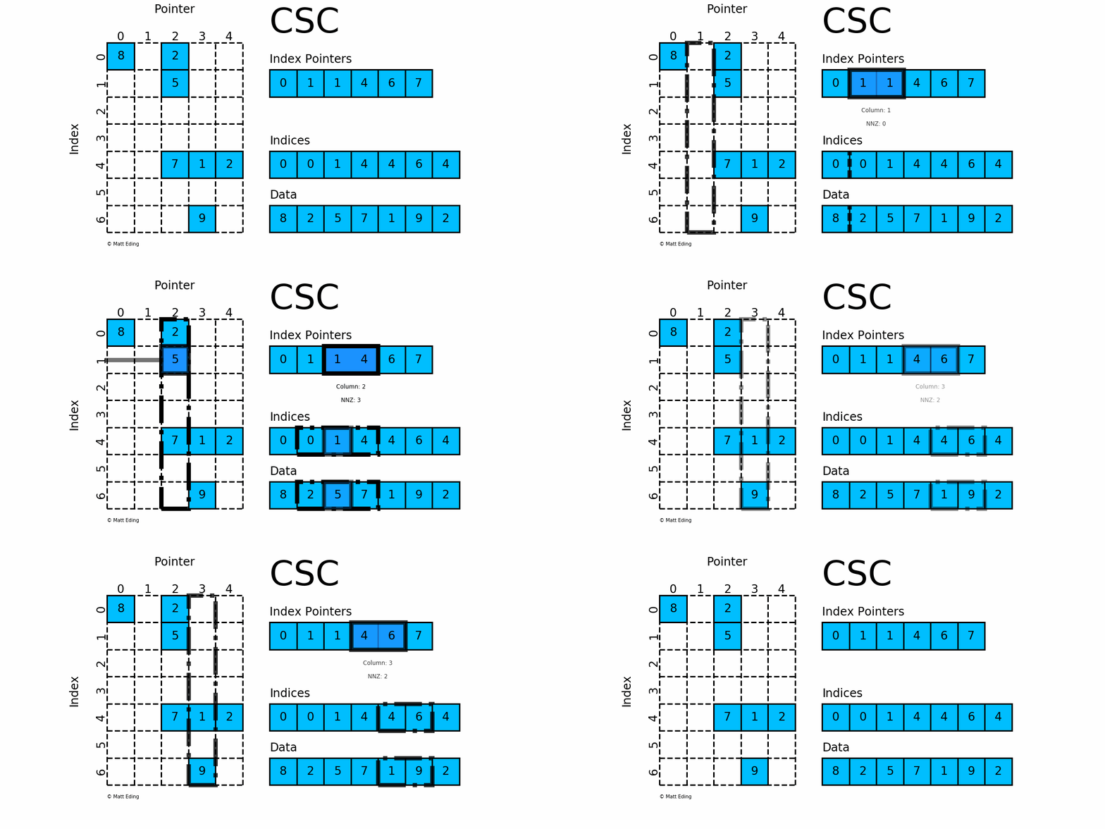
Adjacent pairs of index pointers determine two things. First, their position in the pointer array is the row number. Second, these values represent the [start:stop] slice of the indices array, and their difference is the NNZ elements in each row. Using the pointers, look up the indices to determine the column for each element in the data.
CSC works exactly the same as CSR but has column based index pointers and row indices instead. Below is a diagram of the same data in this format. Notice for this particular case, CSC is slightly more compact with two fewer index pointers.
In [40]: csc = sparse.csc_matrix(csr)  # convert format

In [41]: csc.indptr
Out[41]: array([0, 1, 1, 4, 6, 7], dtype=int32)

In [42]: csc.indices
Out[42]: array([0, 0, 1, 4, 4, 6, 4], dtype=int32)

In [43]: csc.data
Out[43]: array([8, 2, 5, 7, 1, 9, 2], dtype=int64)
As promised, the compressed formats are indeed faster than their COO counterpart. For a modest-sized matrix, we see a 2x speed gain vs COO and 60x speedup vs dense!
In [44]: csr.resize(1000, 1000)

In [45]: %timeit csr @ csr
# 111 µs ± 3.66 µs per loop (mean ± std. dev. of 7 runs, 10000 loops each)

In [46]: coo = csr.tocoo()  # another way to convert

In [47]: %timeit coo @ coo
# 251 µs ± 8.06 µs per loop (mean ± std. dev. of 7 runs, 1000 loops each)

In [48]: arr = csr.toarray()

In [49]: %timeit arr @ arr  # order of magnitude slower!
# 632 ms ± 2.02 ms per loop (mean ± std. dev. of 7 runs, 1 loop each)
Block Sparse Row
Block Sparse Row (BSR) is like CSR but stores sub-matrices rather than scalar values at locations.
In [50]: ones = np.ones((2, 3), dtype=int)

In [51]: data = np.array([ones + i for i in range(4)])

In [52]: indices = [1, 2, 2, 0]

In [53]: indptr = [0, 2, 3, 4]

In [54]: bsr = sparse.bsr_matrix((data, indices, indptr))

In [55]: bsr.todense()
Out[55]:
matrix([[0, 0, 0, 1, 1, 1, 2, 2, 2],
        [0, 0, 0, 1, 1, 1, 2, 2, 2],
        [0, 0, 0, 0, 0, 0, 3, 3, 3],
        [0, 0, 0, 0, 0, 0, 3, 3, 3],
        [4, 4, 4, 0, 0, 0, 0, 0, 0],
        [4, 4, 4, 0, 0, 0, 0, 0, 0]])
This implementation requires all the sub-matrices to have the same shape, but there are more generalized constructs with block matrices that relax this constraint.
These matrices do not have their unique data structure in SciPy, but can be indirectly made via the sparse.bmat constructor function.
In [56]: A = np.arange(8).reshape(2, 4)  # can use dense arrays

In [57]: T = np.tri(5, 4)

In [58]: L = [[8] * 4] * 2  # can use lists

In [59]: I = sparse.identity(4)  # can use sparse arrays

In [60]: Z = sparse.coo_matrix((2, 3))  # zeros to create column gap

In [61]: sp.bmat([[   A,    Z,    L],
    ...:          [None, None,    I],
    ...:          [   T, None, None]], dtype=int)
Out[61]:
<11x11 sparse matrix of type '<class 'numpy.int64'>'
        with 33 stored elements in COOrdinate format>

In [62]: _.toarray()  # ipython previous output
Out[62]:
array([[0, 1, 2, 3, 0, 0, 0, 8, 8, 8, 8],
       [4, 5, 6, 7, 0, 0, 0, 8, 8, 8, 8],
       [0, 0, 0, 0, 0, 0, 0, 1, 0, 0, 0],
       [0, 0, 0, 0, 0, 0, 0, 0, 1, 0, 0],
       [0, 0, 0, 0, 0, 0, 0, 0, 0, 1, 0],
       [0, 0, 0, 0, 0, 0, 0, 0, 0, 0, 1],
       [1, 0, 0, 0, 0, 0, 0, 0, 0, 0, 0],
       [1, 1, 0, 0, 0, 0, 0, 0, 0, 0, 0],
       [1, 1, 1, 0, 0, 0, 0, 0, 0, 0, 0],
       [1, 1, 1, 1, 0, 0, 0, 0, 0, 0, 0],
       [1, 1, 1, 1, 0, 0, 0, 0, 0, 0, 0]])
Diagonal Matrix
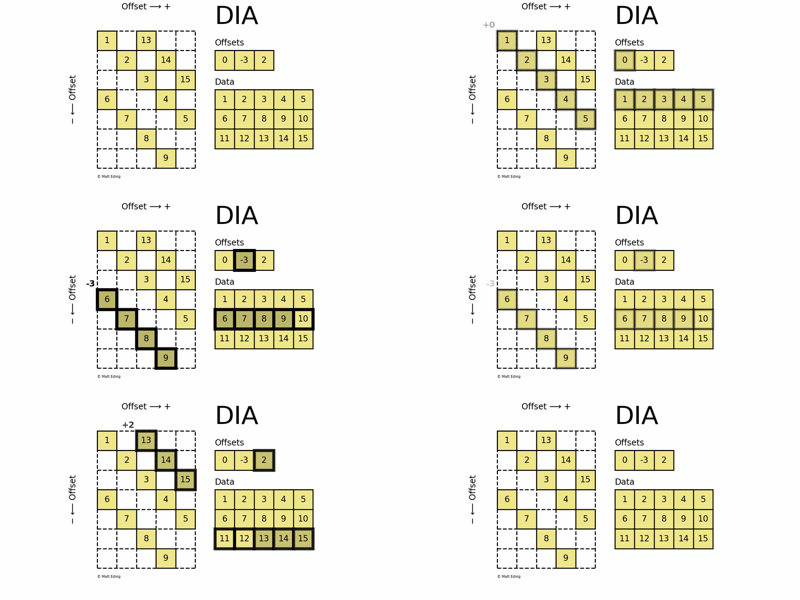
Perhaps the most specialized of the formats to store sparse data is the DIAgonal (DIA) variant. It is best suited for data that appears along the diagonals of a matrix.
In [63]: data = np.arange(15).reshape(3, -1) + 1

In [64]: offsets = np.array([0, -3, 2])

In [65]: dia = sparse.dia_matrix((data, offsets), shape=(7, 5))

In [66]: dia.toarray()
Out[66]:
array([[ 1,  0, 13,  0,  0],
       [ 0,  2,  0, 14,  0],
       [ 0,  0,  3,  0, 15],
       [ 6,  0,  0,  4,  0],
       [ 0,  7,  0,  0,  5],
       [ 0,  0,  8,  0,  0],
       [ 0,  0,  0,  9,  0]])
The data is stored in an array of shape (offsets) x (width) where the offsets dictate the location of each row in the data array along diagonal. Offsets are below or above the main diagonal when negative or positive respectively. Note that if a row in the data matrix is cutoff, the excess elements can assume any value (but they must have placeholders).
In [67]: dia.data.ravel()[9:12] = 0  # replace cutoff data

In [68]: dia.data
Out[68]:
array([[ 1,  2,  3,  4,  5],
       [ 6,  7,  8,  9,  0],
       [ 0,  0, 13, 14, 15]])

In [69]: dia.toarray()  # same array repr as earlier
Out[69]:
array([[ 1,  0, 13,  0,  0],
       [ 0,  2,  0, 14,  0],
       [ 0,  0,  3,  0, 15],
       [ 6,  0,  0,  4,  0],
       [ 0,  7,  0,  0,  5],
       [ 0,  0,  8,  0,  0],
       [ 0,  0,  0,  9,  0]])
Specialized Functions
In addition to the multitude of formats, there is a plethora of functions specialized just for sparse matrices. Use these functions whenever possible rather than their NumPy counterparts, otherwise speed performances will be compromised. Even worse, the resulting calculations could be incorrect!
- inherited methods
- scipy.sparse.spmatrix.mean
- scipy.sparse.spmatrix.getcol
- scipy.sparse.spmatrix.getmaxprint
- …
- general functions
- scipy.sparse.load_npz
- scipy.sparse.isspmatrix_coo
- scipy.sparse.hstack
- …
- linear algebra
- scipy.sparse.linalg.svds
- scipy.sparse.linalg.inv
- scipy.sparse.linalg.norm
- …
- graph algorithms
- scipy.sparse.csgraph.dijkstra
- scipy.sparse.csgraph.minimum_spanning_tree
- scipy.sparse.csgraph.connected_components
- …
Looking into the details of these are left as an exercise to the avid reader.
Other Libraries
SciPy is not the only resource for working with sparse structures in the Python ecosystem. While most appear to use the SciPy package internally, they have all made it their own. I will present several libraries that I find most compelling, but this is not supposed to be the end all be all.
Pandas
Data science today wouldn’t be what it is without Pandas, so it doesn’t come as a surprise that it supports sparse variants of its data structures. A really neat feature is that inferred elements do not have to be forms of 0!
In [70]: import pandas as pd

In [71]: ss = pd.SparseSeries.from_coo(dia.tocoo())

In [72]: ss  # uses a MultiIndex for the coordinates
Out[72]:
0  0     1
   2    13
1  1     2
   3    14
2  2     3
   4    15
3  0     6
   3     4
4  1     7
   4     5
5  2     8
6  3     9
dtype: Sparse[int64, 0]
BlockIndex
Block locations: array([0], dtype=int32)
Block lengths: array([12], dtype=int32)

In [73]: data = dict(A=[np.nan, 1, 2], B=[np.nan, 3, np.nan])

In [74]: sdf = pd.DataFrame(data).to_sparse()

In [75]: type(sdf).mro()  # class inheritance hierarchy
Out[75]:
[pandas.core.sparse.frame.SparseDataFrame,
 pandas.core.frame.DataFrame,
 pandas.core.generic.NDFrame,
 pandas.core.base.PandasObject,
 pandas.core.base.StringMixin,
 pandas.core.accessor.DirNamesMixin,
 pandas.core.base.SelectionMixin,
 object]

In [76]: sdtype = pd.SparseDtype(object, fill_value='e')  # not restricted to null values

In [77]: pd.SparseArray(list('abcdeeeeeeee'), dtype=sdtype)
Out[77]:
[a, b, c, d, e, e, e, e, e, e, e, e]
Fill: e
IntIndex
Indices: array([0, 1, 2, 3], dtype=int32)
Scikit-Learn
The machine learning powerhouse, Scikit-Learn, supports sparse matrices in many areas. This is important since big data thrives on sparse matrices (assuming enough sparsity). After all, who wouldn’t want to have performance gains from these number-crunching algorithms? It hurts having to wait on CPU intensive SVMs, not to mention discovering some data won’t fit into working memory!
Scikit-Learn’s term-document matrices produced by text vectorizers result in CSR matrices. This is crucial for NLP since most words are used sparingly if at all. Naively using a dense format might otherwise cause speed bottlenecks and lots of wasted memory.
In [78]: from sklearn.feature_extraction.text import CountVectorizer

In [79]: bow = CountVectorizer().fit_transform(['demo'])

In [80]: sparse.isspmatrix(bow)
Out[80]: True

In [81]: sparse.save_npz('bag_of_words.npz', bow)  # store for future use
Other areas where Scikit-Learn has the ability to output sparse matrices include:
- sklearn.preprocessing.OneHotEncoder
- sklearn.preprocessing.LabelBinarizer
- sklearn.feature_extraction.DictVectorizer
Moreover there are utilities that play well with sparse matrices such as scalers, a handful of decompositions, some pairwise distances, train-test-split, and many estimators can predict and/or fit sparse matrices. In short embrace their usage whenever possible to make your machine learning models more efficient.
PyData Sparse
As another implementation, PyData’s sparse library provides an interface like np.ndarray instead of np.matrix, permitting creation of multidimensional sparse arrays.
The caveat is that as of the writing of this article, only COO and DOK formats are supported.
In [82]: import sparse as sp  # avoid name clobbering with scipy.sparse

In [83]: sarr = sp.random((3, 4, 2), density=0.2)  # 3-D sparse array

In [84]: sarr
Out[84]: <COO: shape=(3, 4, 2), dtype=float64, nnz=4, fill_value=0.0>

In [85]: sarr += 1  # not possible in scipy.sparse

In [86]: sarr
Out[86]: <COO: shape=(3, 4, 2), dtype=float64, nnz=4, fill_value=1.0>  # fill_value updates!

In [87]: sarr.todense()
Out[87]:
array([[[1.        , 1.        ],
        [1.        , 1.        ],
        [1.        , 1.        ],
        [1.        , 1.        ]],

       [[1.        , 1.        ],
        [1.86024163, 1.        ],
        [1.37233162, 1.1114997 ],
        [1.        , 1.        ]],

       [[1.        , 1.        ],
        [1.        , 1.16850612],
        [1.        , 1.        ],
        [1.        , 1.        ]]])
In SciPy, logical operators are not directly implemented, but AND (&) and OR (|) can be emulated by constraining the dtype to bool:
In [88]: class LogicalSparse(sparse.coo_matrix):  # scipy COO
    ...:    def __init__(self, *args, **kwargs):
    ...:        super().__init__(*args, dtype=bool, **kwargs)  # leverage existing base class
    ...:
    ...:    def __and__(self, other):  # self & other
    ...:        return self.multiply(other)
    ...:
    ...:    def __or__(self, other):  # self | other
    ...:        return self + other
Unfortunately NOT (~) is impossible since it would make a sparse matrix into a dense one (theoretically self - 1).
Until now, that is.
As seen earlier, sparse will dynamically update the fill value to accommodate current states.
In [89]: mask = sp.eye(100, dtype=bool)

In [90]: mask
Out[90]: <COO: shape=(100, 100), dtype=bool, nnz=100, fill_value=False>

In [91]: ~mask
Out[91]: <COO: shape=(100, 100), dtype=bool, nnz=100, fill_value=True>
Final Thoughts
Hopefully this article has enlightened how to use sparse data structures properly so you can go forth and use them with confidence for future projects. Knowing the pros and cons of each format (including dense) will aid in selecting the optimal one for a given task. Be mindful that while sparse matrices are are great tool, they are not necessarily a replacement for arrays. If a matrix is not sufficiently sparse, the multitude of storage arrays behind the scenes will actually take up more resources than a regular dense array would. Furthermore if you need to regularly mutate an array, perform computations in between, and display output, then sparsity simply isn’t worth the trouble. But all these concerns aside, hopefully sparse matrices can help “lighten” your load.
Comparison of Matrix Formats
| COO | DOK | LIL | CSR | CSC | BSR | DIA | Dense | |
|---|---|---|---|---|---|---|---|---|
| indexing | no | yes | yes | yes | yes | no† | no | yes |
| “write-only” | yes | yes | yes | no | no | no | no | yes |
| “read-only” | no | no | no | yes | yes | yes | yes | yes |
| low memory‡ | yes | no | no | yes | yes | yes | yes | no |
| PyData sparse | yes | yes | no | no | no | no | no | n/a |
† BSR raises NotImplementedError: rather than explicitly raising TypeError: 'xxx_matrix' object is not subscriptable. So maybe in the future it will support indexing.
‡ Assuming enough NNZ.
In [92]: exit() # the end :D
Code used to create the above animations is located at my GitHub.