Matt Eding Python & Data Science Blog:
    About     Archive     Feed

Numpy Broadcasting

NumPy - Broadcasting

NumPy has an awesome feature known as broadcasting. This feature allows users to perform operations between an array and another array or a scalar. Conceptually, NumPy expands the arrays until their shapes match (if possible). The rule to determine whether two arrays can be broadcasted is:

Corresponding axes must be equal or 1 when the shapes are right-aligned.

Here is an example of the rule working:

In [1]: import numpy as np

In [2]: arr_1 = np.zeros(shape=(2, 5, 3, 7, 10))

In [3]: arr_2 = np.full(shape=(3, 1, 10), fill_value=np.nan)

In [4]: shapes = [str(a.shape) for a in (arr_1, arr_2)]

In [5]: longest = len(max(shapes, key=len))

In [6]: rjusts = [s.rjust(longest) for s in shapes]

In [7]: print(*rjusts, sep='\n')
# (2, 5, 3, 7, 10)
#       (3, 1, 10)

Looking at the above output:

  • The first two columns do not have corresponding values in the second row. The missing values will be created and expanded into 2 and 5.
  • The middle and last columns have equal values between the two shapes. These axes will not be expanded.
  • The remaining column has values 7 and 1. While the values are not equal, the 1 will be expanded into 7.

Here is an example that fails to broadcast:

In [8]: arr_3 = np.array([[[4, 2, 1]]])

In [9]: arr_4 = (np.linspace(0, 100, 12)  # 12 equally spaced numbers from 0 to 100
   ...:            .reshape(-1, 6)  # -1 has numpy calculate first axis dimension
   ...:            .astype(int))

In [10]: arr_3 - arr_4
# ValueError: operands could not be broadcast together with shapes (2,6) (1,1,3)

With shape (1, 1, 3), the two 1’s are ok since the first has no corresponding value and the second is a 1. It is the final axis with 6 and 3 that cause the error; they are not equal and neither are 1. NumPy will not venture to guess whether it should double the 3 to a 6. If this is what you wanted, you would need to manually extend them:

In [11]: np.dstack((arr_3, arr_3)) - arr_4  # stack extra copy depth-wise
Out[11]:
array([[[  4,  -7, -17, -23, -34, -44],
        [-50, -61, -71, -77, -88, -99]]])

In [12]: _.shape  # ipython previous output
Out[12]: (1, 2, 6)

While the notion of expansion is helpful to understand broadcasting, NumPy does not actually create new, bigger arrays. This allows NumPy to be more efficient in both speed…

In [13]: nums = np.arange(1e6).reshape(10, 10, -1)  # -1 has numpy calculate third axis dimension

In [14]: ones = np.ones_like(nums)  # same shape with np.*_like functions

In [15]: %timeit nums + 1
# 1.01 ms ± 5.15 µs per loop (mean ± std. dev. of 7 runs, 1000 loops each)

In [16]: %timeit nums + ones
# 1.14 ms ± 8.1 µs per loop (mean ± std. dev. of 7 runs, 1000 loops each)

… and memory since an array of only unique values needs to allocate space for all the values (even when taking dtypes into consideration).

In [17]: (1).__sizeof__()
# 24

In [18]: ones.__sizeof__()
# 800128

In [19]: np.array_equal(nums + 1, nums + ones)
Out[19]: True

Below is an example of adding a scalar to a 3D array:

In [20]: arr_3d = np.arange(60).reshape(5, 3, 4)

In [21]: np.shape(arr_3d)
Out[21]: (5, 3, 4)

In [22]: np.shape(1)
Out[22]: ()

In [23]: result = arr_3d + 1

In [24]: np.shape(result)
Out[24]: (5, 3, 4)
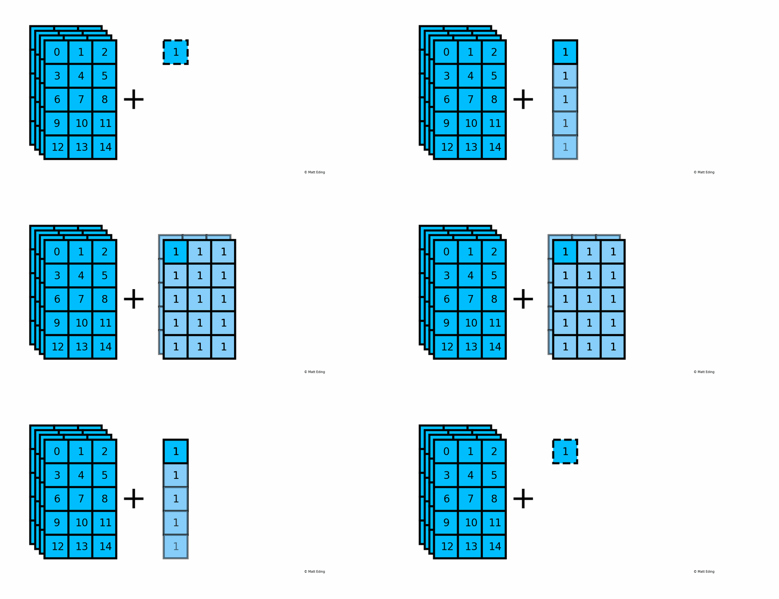
Broadcasting-3D-Scalar

Another example with multiplying a column by a row:

In [25]: np.c_[0:3]  # create column with slice syntax
Out[25]:
array([[0],
       [1],
       [2]])

In [26]: np.r_[0:4]  # create row with slice syntax
Out[26]: array([0, 1, 2, 3])

In [27]: _ * __  # ipython previous two outputs
Out[27]:
array([[0, 0, 0, 0],
       [0, 1, 2, 3],
       [0, 2, 4, 6]])

Broadcasting-Column-Row

An application in data science using broadcasting is the ability to normalize data to range from 0 to 1.

In [28]: data = np.array([[ 4.4,  2.1, -9.0],
    ...:                  [ 0.4, -3.2,  3.9],
    ...:                  [-6.7, -5.0,  7.4]])

In [29]: data -= data.min()  # make min value 0

In [30]: data /= data.max()  # make max value 1

In [31]: assert (data.min() == 0) and (data.max() == 1)

In [32]: data
Out[32]:
array([[0.81707317, 0.67682927, 0.        ],
       [0.57317073, 0.35365854, 0.78658537],
       [0.1402439 , 0.24390244, 1.        ]])

Hopefully this will help you embrace using the power of broadcasting in your future work. It allows you to concisely write code (i.e. less error prone) while making your program more performant at the same time.

In [33]: exit()  # the end :D

Code used to create the above animations are located at my GitHub.

Dde Summarizer P2

Discrete Differential Evolution Text Summarizer

Part 2

In Part 1, we introduced metrics to use for determining how similar sentences are using Jaccard, and ways to measure how well clusters are distinguished from one another. Now we will go over the process to create the summary using DDE.

First, a random population is generated where each chromosome is made into a partition of clusters. Each cluster represents a topic a given sentence is assigned.

#: make a chromosome that is a random partition with each cluster
clusters = np.arange(summ_len)
chrom = np.full(len(document), -1)
#: ensure that each cluster is accounted for at least once
idxs = np.random.choice(np.arange(len(chrom)), summ_len, replace=False)
chrom[idxs] = np.random.permutation(clusters)
#: fill rest randomly
idxs = (chrom == -1)
chrom[idxs] = np.random.choice(clusters, np.sum(idxs))

For example if there were 10 sentences and we want 3 sentence summary, a possible chromosome in the population could be:
Sentence: [0, 1, 2, 3, 4, 5, 6, 7, 8, 9]
Chromosome: [0, 2, 2, 1, 0, 1, 0, 2, 1, 1]
From this we can see that topic 0 includes sentences 0, 4, and 6. Over time as the algorithm evolves, these topic assignments will change in accordance to how well their fitness metrics perform. After a desired amount of generations, we will pick representative sentences from each cluster to use in the summary.

With evolutionary algorithms, at each step we generate an offspring population using the parent population. The way DDE works, we sample three distinct chromosomes from the parent population (x_1, x_2, and x_3) to derive a new chromosome. This is defined as x_1 + lambda(x_2 - x_3) where lambda is a scale factor chosen by the user. To ensure it is discrete, we store the result in a numpy array with an integer dtype and also use modulo by the number of clusters to keep the number of desired summary sentences constant. Below is a vectorized version to apply to the entire population array at once:

n = np.arange(len(pop))
s = frozenset(n)
#: get 3 distinct chromosomes that differ from i_th chromosome
idxs = np.array([np.random.choice(tuple(s - {i}), size=3, replace=False) for i in n])
chrom_1, chrom_2, chrom_3 = map(np.squeeze, np.split(pop[idxs], 3, axis=1))
#: discrete differential evolution
offspr = (chrom_1 + lambda_ * (chrom_2 - chrom_3)) % summ_len

For each parent/offspring pairing, we keep the better fit one according to its cohesion_separation score (see part 1) by overriding the population array in place. As this is the main bottleneck, use multiprocessing to utilize all the cores on your machine.

#: determine whether parents or offspring will survive to the next generation
with multiprocessing.Pool() as pool:
    fits = pool.map(cohesion_separation, itertools.chain(pop, offspr))
i = len(pop)
fit_pop, fit_off = fits[:i], fits[i:]
mask = fit_off > fit_pop
pop[mask] = offspr[mask]

Finally the new population is mutated according to a random state created anew for each generation. For each chromosome, genes are randomly selected for crossover–dubbed as such to mimic real life chromosomal inversion. Those selected genes have their order reversed while other ones are kept in place. Below is the code to apply this operation in vectorized form. Unfortunately I could not figure out a clearer way to achieve this without explicit for loops.

rand = np.random.random_sample(pop.shape)
mask = rand < sigmoid(pop)
#: inversion operator -> for each row reverse order of all True values
idxs = np.nonzero(mask)
arr = np.array(idxs)
sorter = np.lexsort((-arr[1], arr[0]))
rev = arr.T[sorter].T
pop[idxs] = pop[(rev[0], rev[1])]

This process is repeated for a fixed number of generations. After many iterations, DDE gravitates towards optimal solutions as only most fit survives. In the 3rd and final installment, we will go over how to extract the representative sentences resulting from the evolutionary process to create the summary.

For the full implementation feel free to look at my EvolveSumm repository on GitHub.